Causal relations as processes

Rottman and Hastie use the term ‘causal relationships’ to refer to causality; here, we treat them as processes and structures. Rottan and Haustie did not set out to be exhaustive; rather, they wished to highlight a few fallacies, and in that respect their contribution was certainly very useful. In their analysis, they identify five forms of causal relationships. See their overview below:

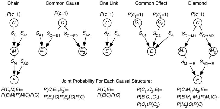
As you can see at the bottom, the authors also consider the likelihood of causal relationships. For the visualisation of causation, we limit ourselves to proven causal processes. We use only the conjunction from formal logic, or the union from set theory, as an operator between different causal structures. See the example of the raincycle. The exclusive ‘OR’ can also be used between structures, but not within structures themselves.

In this concept the pocess notation is the formal basis of the graphs that visualise causality. The process description consists of a brief description of the process, or the measured result of the process for directed weighted graphs, followed by two numbers in square brackets, separated by a comma. These numbers show how the process evolves over time: from one node to the next. If the exact time is known, they can also serve as a time indicator, but in that case the unit of time used must be specified in the label. This is followed by an equals sign. Next come the brief descriptions of the two nodes, each followed by a number in square brackets, separated by an operator. These numbers must correspond, in each case, to the first number and the second number in the process description, respectively.

Four of these causal relationships identified by Rottman and Hastie correspond to structures that we ourselves propose. 'One Link' corresponds with the graph of 1 process, 'Chain' corresponds with concatenation of processes, 'Common Cause' with convergence of processes en 'Common Effect' met divergence of processes. The 'Diamond' structure is the combination of convergence en divergence in our mapping. And as you can see in our example, it can also take the form of a triangle. See ‘infiltration’. So we’ll drop this one, but we’ll add three more structures: Interaction, Circularity and Feedback. These structures are apparently not suitable for investigating Bayesian probabilistic causal networks. Butz, Cory, Yan, Wen, Yang and Boting also limit themselves to the same structures as Rottan and Haustie (Butz, Cory, Yan, Wen, Yang, Boting, 2025).

By classifying necessity under the common umbrella of processes, whilst excluding stochastic processes, we are able to disregard the speculative element, which nevertheless always involves probability. A stochastic process is a sequence of random outcomes. Unlike a deterministic process, the outcomes are not known in advance. The stochastic process is described by a sequence of random states and their associated joint probability distribution.

In process notation, we use the operator “►” for causation. The operator connects the state that existed before a causal action took place and the state after the action. For actions that simply follow one another without being necessary, sequential actions, we use the operator “»”. For processes where energy is continuously exchanged, the operator “→” is used. Because, in terms of its continuity, it is a specific form of causality, we use a specific operator even when discussing causality. In ecological systems, this exchange of energy is essential for survival.

Since, when visualising processes, we are concerned solely with proven necessity or a sequence of actions that, whilst not necessarily so, have been empirically verified, we can omit the speculative qualifier ‘possible to occur’. We therefore do not use stochastic variables, or indeed any variables at all. We thus also move away from the algebraic representation of reality. This makes it possible to use these graphs in both the humanities and the arts, as well as in technical and vocational education. In this way, science can still be covered in these subjects without the need for extensive knowledge of mathematics.

Themore for causality formal logic with the inclusive ‘OR’ can not be used. It would lead to a lot of ambiguities (Bernstein, 2019;Beckers, Vennekens, 2017). We want the visualisations to be unambiguous. We therefore base our work on Kripke’s semantics for modal logic, which is briefly summarised below.

A Kripke frame, or modal frame, is a pair (W, R) where W is a non-empty set and R is a binary relation on W. Elements of W are called nodes or worlds, and R is known as the accessibility relation.

A Kripke model is a triplet (W, R, ⊩) where (W, R) is a Kripke frame and ⊩ is a relation between nodes of W and modal formulas.

Alongside possibility and probability, causality is a component of modal logic. There are quite a few differences compared with formal logic:

(1) A causal relationship implies a logical implication, but not vice versa
(p □→ q) →(p → q)
This reads as “if q is a necessary consequence of p, then p implies q”.

(2) Whilst formal logic appears to be timeless, causality is bound to time (David Hume). The effect follows the cause.

(3) Modal logic does not have truth tables, but it does have decision procedures.

(4) Causality can be represented by a directed graph.

“Our basic idea is simply this: we describe properties of directed graphs consisting of points (‘possible worlds’ if you like grandeur) with directed links encoded in an ‘accessibility relation’ between points. A universal modality □ Ø is true at a point in a graph if Ø is true at all points reachable by a directed arrow.” (van Benthem, IEP)

(5) The main decision-making procedure for establishing causality is the ‘counterfactual’ test. Schürman defined the test in the context of the ‘Why-Because’ analysis (WBA).

“To check the correctness of a cause-and-effect relationship, the Counterfactual Test (CT), based on work of David Lewis and David Hume, is used. "If the (potential) causal factor had not occurred, could the effect have occurred?" If this test is answered with "no", then the potential causal factor is a "necessary causal factor" (abbr. NCF). Use of the CT ensures that all nodes in the WBG are correctly linked.” (Schürmann, WBA)

An example to illustrate the reliance on the ‘counterfactual’ test. The formation of rain clouds depends on the presence of atmospheric condensate consisting of water vapour and ice crystals above the freezing point. When the air cools to the dew point and becomes saturated, water vapour normally condenses into cloud droplets. This condensation usually takes place on condensation nuclei such as salt or dust particles that are small enough to be suspended in the air by normal air circulation.

So you need clouds in order for rain clouds to form. The rain falls through the base of the rain cloud after droplets of 20 microns have grown to 2,000 microns through collisions during the up-and-down movement of droplets and ice crystals. The rain therefore depends on the presence of those clouds. We therefore have unambiguous transitivity here. If those clouds had not been there, it would not have rained.

This ‘counterfactual’ test is also found in legal reasoning. In that context, ‘conditio sine qua non’ is a commonly used term (Stepanov, 1985). It means that we conclude that ‘A caused B’ if ‘had A not occurred, B would not have occurred’. When using disjunction, this rule can lead to paradoxes.

(6) Whilst implication is transitive, transitivity is disputed in the case of causality. In classical logic, if X implies Y and Y implies Z, then X also implies Z. In the case of causal relationships, every relationship must be subjected to the ‘counterfactual test’, including that between X and Z.

A comprehensive discussion of modal logic can be found on Wikipedia under the entry: Kripke semantics.

References

Beckers, Sander and Joost Vennekens, 2017, The Transitivity and Asymmetry of Actual Causation, Ergo: An Open Access Journal of Philosophy, volume 4, pp 1-27. <https://quod.lib.umich.edu/e/ergo/12405314.0004.001/--transitivity-and-asymmetry-of-actual-causation?rgn=main;view=fulltext>.

Bernstein, Sara. (2019). Lewis’s Theories of Causation and Their Influence. 10.1017/9781316779651.015., <https://sarajbernstein.github.io/sjb/LewisTCTI.pdf>.

Butz, Cory & Yan, Wen & Yang, Boting. (2005). The Computational Complexity of Inference Using Rough Set Flow Graphs. 10.1007/11548669_35. <https://surl.li/jyzfcj>.

Müller, A. (2000). Eine kurze Geschichte des BCL: Heinz von Foerster und das Biological Computer Laboratory. Österreichische Zeitschrift für Geschichtswissenschaften, 11(1), 9–30. https://doi.org/10.25365/oezg-2000-11-1-2 <https://constructivist.info/radical/papers/mueller/mueller00-bcl.html>.

Rottman BM, Hastie R. Reasoning about causal relationships: Inferences on causal networks. Psychol Bull. 2014 Jan;140(1):109-39. doi: 10.1037/a0031903. Epub 2013 Apr 1. PMID: 23544658; PMCID: PMC3988659. <https://pmc.ncbi.nlm.nih.gov/articles/PMC3988659/>.

Schürmann, Tim, (WBA) 'Counterfactual Test’, Workgroup RVS, Faculty of Technology, Bielefeld University) <https://rvs-bi.de/research/WBA/IntroWBA-ENG.pdf>.

van Benthem, Johan, (IEP), Modal Logic: A Contemporary View, University of Amsterdam, Stanford University, and Tsinghua University, The Netherlands, U. S. A., and China, <https://iep.utm.edu/modal-lo/>

Kripke, Saul (1963). Semantical Considerations on Modal Logic. Acta Philosophica Fennica 16:83-94.

Stepanov, Alexander (1985), Towards a Theory of Causal Implication, Department of Electrical Engineering and Computer Science, Polytechnic University of New York, 1985, <https://surl.li/lsdoni >